Training a model to detect deepfake audio

Part 2/2: Building the training pipeline that returns REAL / FAKE results on audio inputs

In the last article, we took the first real step toward building a reliable fake audio detector.

By combining real-world audio from ASVspoof 2019 with synthetic data from Orpheus, we created a balanced dataset that mirrors the complexity of real scenarios.

We also explored key audio augmentations like time shifts, noise, pitch changes, and gain to help the model adapt to unpredictable inputs. And with Mel spectrograms and masking, we pushed it to learn beyond surface-level patterns and spot deeper fake cues.

To ground this work in real-world context, we also brought in expert insight from Silviu Gresoi: AI, ML & Anti-Fraud Specialist with over 20 years of experience across banking, energy, insurance, and pharma.

His perspective helped highlight the growing impact of AI-driven fraud and the urgent need for effective detection tools.

If you haven’t read it yet, make sure to check out Part 1 it sets the foundation for everything we’re diving into today.

---

Table of contents

1. Training the model

2. Final results

3. Conclusions

---

Key takeaways

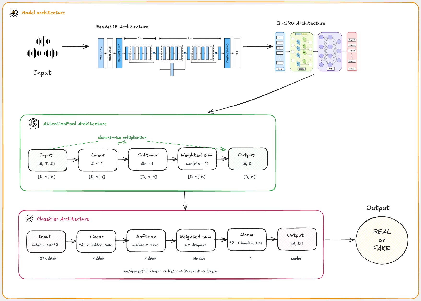
• We’ll be using a pre-trained ResNet18 model with Bi-GRU to classify the audio.

• How we got to 95-97% precision & recall in less epochs, what worked and what didn’t.

• How to build a Streamlit app that allows real-time inference: users upload audio files, which are preprocessed and classified as REAL or FAKE with confidence scores.

1. Training the model

Now comes the hard part: creating the model.

We need a model that can detect deepfake audio files. It is important to understand from the outset that our dataset is image-based.

Although we are talking about audio files, our final dataset is actually a spectrogram of our audio file, which is basically an image of the audio.

This means that our solution must use a convolutional approach. Our final answer, however, needs to have only two values: False (0) or True (1).

For this reason, I have chosen ResNet18 as the convolutional backbone, due to its strong performance on visual tasks and the availability of pre-trained weights, which help to accelerate convergence and improve generalisation, even when applied to spectrogram-like audio inputs.

To illustrate this, I will give you an example: Imagine you want to teach two children, aged 1 and 2, how to wash their hands. Of course, you can teach both of them, but even though they both don't know how to do this, the 2-year-old will learn faster than the 1-year-old.

This can be applied to our situation as well: even though ResNet18 was trained on a specific dataset (ImageNet) that didn't contain any spectrograms, it will adapt more quickly to the new dataset than if we only used the basic implementation without any prior training.

However, spectrograms also contain important temporal information — how sound patterns evolve over time. To capture these sequential dependencies, I integrated a Bi-GRU after the ResNet backbone, allowing the model to learn both past and future context within the time axis of the spectrogram.

Once the Bi-GRU has processed the temporal sequence of features, we require a mechanism that can focus on the most informative time steps. For this, I use an Attention Pooling layer, which learns to assign different weights to each time step, effectively telling the model what parts of the sequence to pay more attention to.

This allows the network to focus on what's important and ignore what isn't.

Finally, the output of the Attention Pooling layer is passed to a simple classification head — a small fully connected neural network — that outputs a single value between 0 and 1, representing the probability that the input audio is fake.

This makes the architecture suitable for binary classification tasks.

Now that we have a well-established model, we can define a process and write the code that follows it.

import torch
import torch.nn as nn
import torch.nn.functional as F
from torchvision import models

class AttentionPool(nn.Module):
    def __init__(self, in_dim):
        super().__init__()
        self.attn = nn.Linear(in_dim, 1)

    def forward(self, x):
        # x: [B, T, D]
        scores = self.attn(x)              # [B, T, 1]
        weights = F.softmax(scores, dim=1) # [B, T, 1]
        return (weights * x).sum(dim=1)    # [B, D]

class CRNNWithAttn(nn.Module):
    def __init__(self,  pretrained=True, hidden_size=128, num_layers=1, dropout=0.2):
        super().__init__()
        # 1. Pretrained ResNet18
        if pretrained:
          resnet = models.resnet18(weights='DEFAULT')
        else:
          resnet = models.resnet18()
        # Adapt first conv to accept 1-channel input
        w = resnet.conv1.weight.data.clone()
        resnet.conv1 = nn.Conv2d(2, 64, kernel_size=7, stride=2, padding=3, bias=False)
        resnet.conv1.weight.data[:, 0] = w[:, 0]
        # Remove final pooling & fc
        self.backbone = nn.Sequential(*list(resnet.children())[:-2])

        # 2. Bi-GRU for temporal modeling
        self.gru = nn.GRU(
            input_size=512,          # ResNet last block outputs 512 channels
            hidden_size=hidden_size,
            num_layers=num_layers,
            batch_first=True,
            bidirectional=True,
            dropout=dropout if num_layers>1 else 0.0
        )

        # 3. Attention pooling
        self.attn_pool = AttentionPool(hidden_size*2)

        # 4. Classification head
        self.classifier = nn.Sequential(
            nn.Linear(hidden_size*2, hidden_size),
            nn.ReLU(inplace=True),
            nn.Dropout(dropout),
            nn.Linear(hidden_size, 1)
        )

    def forward(self, x):
        # x: [B, 1, F, T]
        feat = self.backbone(x)            # [B, 512, F', T']
        feat = feat.mean(dim=2)            # collapse freq → [B,512,T']
        feat = feat.permute(0,2,1)         # → [B,T',512]

        out, _ = self.gru(feat)            # → [B,T',2*hidden_size]
        pooled = self.attn_pool(out)       # → [B,2*hidden_size]
        return self.classifier(pooled)     # → [B,1]


# Create the model and put it on the GPU if available
myModel = CRNNWithAttn()
device = torch.device("cuda:0" if torch.cuda.is_available() else "cpu")
myModel = myModel.to(device)
# Check that it is on Cuda
next(myModel.parameters()).device

Getting to train the model

We have now arrived at the most important part: training.

All that’s left is implement the training algorithm, for which we require an appropriate loss function, an optimiser and a real-time learning rate scheduler to help us improve generalisation and convergence.

For the loss function we will choose the binary cross-entropy loss function (or BCEWithLogitsLoss) because it suits our needs best, especially given that we are performing a binary classification.

For the optimizer we will choose Adam, because it is the most widely used optimizer and combines the advantages of both AdaGrad and RMSProp. It provides adaptive learning rates for each parameter and incorporates momentum to accelerate convergence, which is especially useful for problems involving sparse gradients or noisy data.

And for the real-time learning rate scheduler, we will use OneCycleLR, which is simple to implement and, as I mentioned earlier, improves generalisation and convergence. It simply increases the learning rate to a maximum value and then decreases it gradually over the course of training.

Gathering all things up, we get the following implementation for the training phase:

import torch.nn as nn
import torch.nn.functional as F
from torch.utils.data import DataLoader, random_split
from torch.utils.tensorboard import SummaryWriter
from tqdm.auto import tqdm

def training(model, full_dataset, batch_size=32, num_epochs=20,
             val_split=0.2, patience=3, log_dir="runs/exp1"):

    # ── Prepare data loaders ───────────────────────────────────────────────────
    dataset_size = len(full_dataset)
    val_size     = int(val_split * dataset_size)
    train_size   = dataset_size - val_size
    train_ds, val_ds = random_split(full_dataset, [train_size, val_size])

    train_dl = DataLoader(train_ds, batch_size=batch_size, shuffle=True,  num_workers=4)
    val_dl   = DataLoader(val_ds,   batch_size=batch_size, shuffle=False, num_workers=4)

    # ── Loss, Optimizer, Scheduler ────────────────────────────────────────────
    criterion = nn.BCEWithLogitsLoss()
    optimizer = torch.optim.Adam(model.parameters(), lr=1e-3)
    scheduler = torch.optim.lr_scheduler.OneCycleLR(
        optimizer,
        max_lr=1e-3,
        steps_per_epoch=len(train_dl),
        epochs=num_epochs,
        anneal_strategy='linear'
    )

    # ── TensorBoard writer ─────────────────────────────────────────────────────
    writer = SummaryWriter(log_dir)

    # ── Early stopping vars ────────────────────────────────────────────────────
    best_val_acc = 0.0
    epochs_no_improve = 0

    device = next(model.parameters()).device

    # Precompute ImageNet stats tensors for normalization
    imagenet_mean = torch.tensor([0.485, 0.456], device=device).view(1, 2, 1, 1)
    imagenet_std  = torch.tensor([0.229, 0.224], device=device).view(1, 2, 1, 1)

    for epoch in range(1, num_epochs + 1):
        model.train()

        # Epoch-level progress bar
        epoch_bar = tqdm(train_dl, desc=f"Epoch {epoch}/{num_epochs}", unit="batch")

        running_loss = 0.0
        epoch_loss   = 0.0
        correct_preds = 0
        total_preds   = 0

        for inputs, labels in epoch_bar:
            inputs = inputs.to(device)
            labels = labels.to(device).unsqueeze(1).float()

            # normalize to ImageNet stats for pretrained ResNet backbone
            inputs = (inputs - imagenet_mean) / imagenet_std

            optimizer.zero_grad()
            outputs = model(inputs)
            loss = criterion(outputs, labels)
            loss.backward()
            optimizer.step()
            scheduler.step()

            running_loss += loss.item()
            epoch_loss   += loss.item()

            preds = (torch.sigmoid(outputs) > 0.5).float()
            correct_preds += (preds == labels).sum().item()
            total_preds   += preds.size(0)

            # Update the bar’s postfix with live metrics (average over all seen samples)
            epoch_bar.set_postfix({
                "loss": f"{running_loss / total_preds:.4f}",
                "acc":  f"{correct_preds / total_preds:.4f}"
            })

        train_acc  = correct_preds / total_preds
        train_loss = epoch_loss / len(train_dl)

        # —— Validation ——
        model.eval()
        val_loss     = 0.0
        val_correct  = 0
        val_total    = 0

        with torch.no_grad():
            for inputs, labels in val_dl:
                inputs = inputs.to(device)
                labels = labels.to(device).unsqueeze(1).float()
                inputs = (inputs - imagenet_mean) / imagenet_std

                outputs = model(inputs)
                val_loss    += criterion(outputs, labels).item()
                preds        = (torch.sigmoid(outputs) > 0.5).float()
                val_correct += (preds == labels).sum().item()
                val_total   += preds.size(0)

        val_loss = val_loss / len(val_dl)
        val_acc  = val_correct / val_total

        # — Log to TensorBoard —
        writer.add_scalar('Loss/train', train_loss, epoch)
        writer.add_scalar('Acc/train',  train_acc,  epoch)
        writer.add_scalar('Loss/val',   val_loss,   epoch)
        writer.add_scalar('Acc/val',    val_acc,    epoch)

        print(f"Epoch {epoch:02d}  Train Loss: {train_loss:.4f}  Train Acc: {train_acc:.4f}  "
              f"Val Loss: {val_loss:.4f}  Val Acc: {val_acc:.4f}")

        # —— Early Stopping & Checkpointing ——
        if val_acc > best_val_acc:
            best_val_acc = val_acc
            epochs_no_improve = 0
            torch.save(model.state_dict(), f"best_model{epoch}.pth")
            print(f"→ New best model saved (Val Acc: {best_val_acc:.4f})")
        else:
            epochs_no_improve += 1
            if epochs_no_improve >= patience:
                print(f"Early stopping after {epoch} epochs "
                      f"(no improvement in {patience} epochs).")
                break

    writer.close()
    print("Training complete. Best Val Acc: {:.4f}".format(best_val_acc))


num_epochs=10   # Just for demo, adjust this higher.
training(myModel, full_augmented_dataset, num_epochs = num_epochs)

I’ve added a simple progress bar to monitor how the model improves over time.

---

2. Final results

The only thing left to do now is to create a simple interface where we can test our inferences and see how our model performs.

For this the following flow diagram comes in handy:

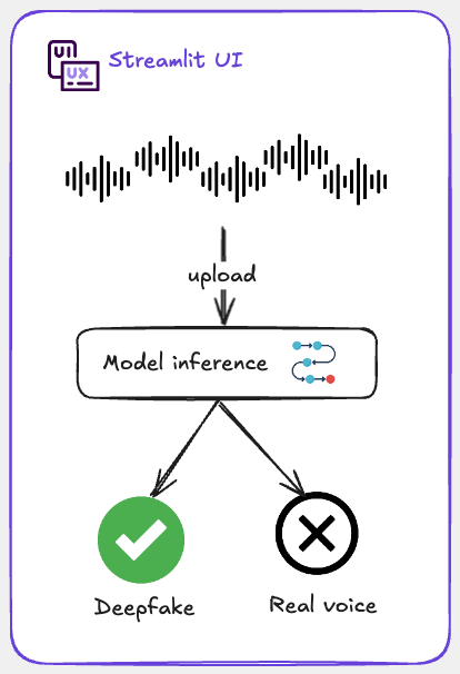
The concept is simple.

We will load the saved .pth file from our trained model, deploy it within a Streamlit app and create a basic graphical interface.

Users can upload a audio file, click a button to analyse it and instantly receive a 'REAL' or 'FAKE' prediction.

And just like that, you've got a deepfake voice detector ready to go!

For this implementation you have the following code sample.

import streamlit as st
from pathlib import Path

# Load your model
@st.cache_resource
def load_model(Model):
    Model.load_state_dict(torch.load('best_model10.pth', map_location=device))
    Model.eval()
    return Model

model = load_model(myModel)

# ImageNet normalization stats (for 1 channel input)
imagenet_mean = torch.tensor([0.485, 0.456], device=device).view(1, 2, 1, 1)
imagenet_std  = torch.tensor([0.229, 0.224], device=device).view(1, 2, 1, 1)

# Audio preprocessing
def preprocess(waveform, sample_rate):
    # Resample if needed
    if sample_rate != 16000:
        resample = T.Resample(orig_freq=sample_rate, new_freq=16000)
        waveform = resample(waveform)

    # Stereo
    if waveform.shape[0] > 1:
        waveform = waveform.repeat(2, 1)

    # Trim / pad to 4 seconds
    max_len = 16000 * 4
    if waveform.shape[1] > max_len:
        waveform = waveform[:, :max_len]
    elif waveform.shape[1] < max_len:
        pad_len = max_len - waveform.shape[1]
        waveform = torch.nn.functional.pad(waveform, (0, pad_len))

    # Convert to MelSpectrogram
    mel_spec = T.MelSpectrogram(
        sample_rate=16000,
        n_fft=780,
        hop_length=195,
        n_mels=64
    )(waveform)
    mel_spec = T.AmplitudeToDB(top_db=80)(mel_spec)

    # Normalize
    mel_spec = (mel_spec - imagenet_mean) / imagenet_std
    return mel_spec

# UI layout
st.title("Audio Classifier: REAL or FAKE")

uploaded_file = st.file_uploader("Upload a .wav/.flac file", type=["wav", "flac"])

if uploaded_file is not None:
    # Load and preprocess
    waveform, sample_rate = torchaudio.load(uploaded_file)
    input_tensor = preprocess(waveform, sample_rate).unsqueeze(0)

    # Inference
    with torch.no_grad():
        output = model(input_tensor)
        prob = torch.sigmoid(output).item()
        label = "REAL" if prob > 0.5 else "FAKE"

    # Display
    st.audio(uploaded_file, format="audio/wav")
    st.markdown(f"### Prediction: **{label}**")
    st.markdown(f"Confidence: `{prob:.2f}`")

Here you have it, a fully working deepfake voice detector that you can play with.

---

3. Results

Future work and Open problems

Now that we have managed to implement the detector, let's address some of the outstanding issues.

One of the most significant issues is the detection of false positives; the model lacks generalisation when it comes to true audio files, which is a step back.

For this problem, I have come up with an improvement that might resolve it.

I’ve made a diagram to help us understand this solution more easily.

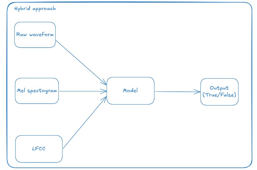
The idea is simple: we just want to implement a hybrid approach.

This approach involves taking different types of features from our audio file and providing them to the model, so that the model can gain a broader perspective on real versus fake audio.

To achieve this, I believe it would be most effective to use raw waveforms, as this would prevent any information from being lost during the transformation into a Mel spectrogram. Additionally, we could utilise Mel spectograms and LFCCs, which could provide us with valuable insights into the audio file.

Another improvement would be to combat a GAN. When we talk about production, we talk about very important information that we don't want to lose.

However, hackers have become more sophisticated because they use GANs to attack systems and bypass the detection layer. I have found a method that can combat such an attack.

When it comes to attacks like this, there are three types of attacks that the hacker can use:

1. Black box attack: where the attacker doesn’t know anything about the victims model or dataset.(we are not interested in this type of attack)

2. Gray box attack: where the attacker knows something about the victims model or dataset(this is what we want to combat)

3. White box attack: where the attacker knows everything about the victims model and dataset(our approach might combat this problem as well, but this is not clear yet)

And for this problem I’ve made another diagram so that is easier for us to follow.

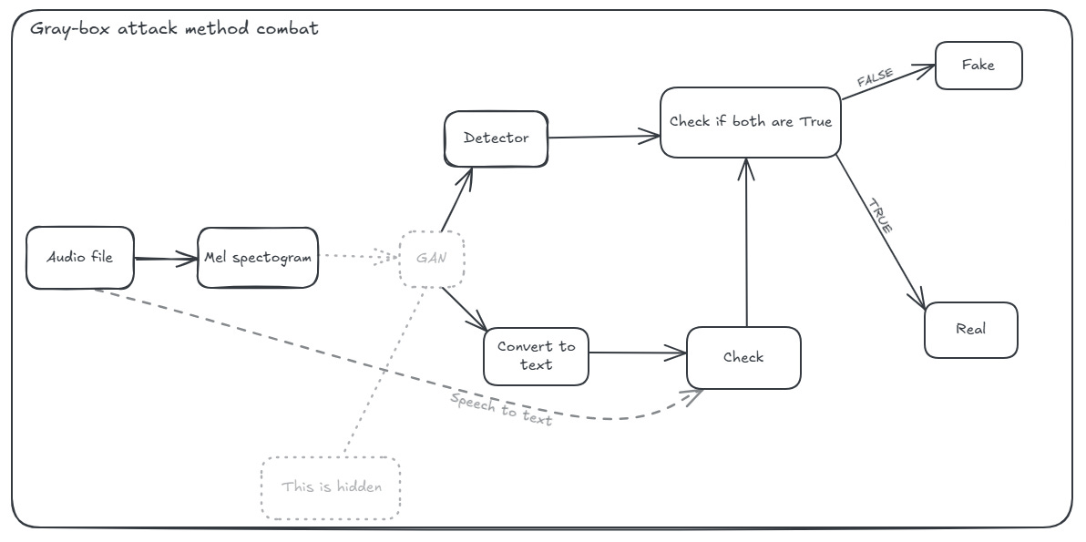
The idea is simple.

We just want to perform a second verification before predicting whether our input is fake or true. We do this by transforming the Mel spectrogram generated by the GAN into text, verifying whether it is equal to the text of the input audio file or empty (i.e. whether it contains text or is just noise).

If they don't coincide, we mark it as fake; otherwise, we mark it as true.

Why does this work? It works because we perform an additional check to verify whether our output is indeed a real audio file. GANs distort the output in such a way that our detector thinks it is a real audio file, even though it is not.

Therefore, the verification works because it will not pass the check.

🔗 Check out the code on GitHub and support us with a ⭐️