Audio deepfake fraud detection system

Part 1/2: Using Spectogram AI and making the most out of the dataset

We’ve made some changes, new name, new logo but there’s more.

Our articles will still cover real problems we’ve faced, just like before, but now with deeper insight and expert input who bring new perspectives and knowledge beyond our own.

The break gave us time to improve and connect with people who know more, so we can offer better insights and support.

This newsletter is a growing community. And our Discord? It’s the place to talk, share, and get the help you need.

---

Key takeaways

• A combination of real world (ASV Spoof 2019) and generated (Orpheus) datasets are needed for a balanced real/fake data if we want a reliable system.

• Augmentations like time shift, noise, pitch shift, and gain are great for improving model performance against varied audio inputs.

• Mel spectrograms extraction combined with masking helps the model generalize beyond obvious deepfake artifacts.

---

📱 [Phone rings]
📳 Riiing... Riiing...

👤 (picks up):
"Hello?"

🤖:
🎉 "Congratulations! You have won a free prize! Just give us your details to claim it..."

👤:
"Yeah... no thanks."

📞 📴 [Call ended]
Click.

Everyone’s had an interaction like the one above, when a random number calls out of nowhere, and your first thought is:

"Is this important... or just another scam?"

You answer cautiously, only to be met with the same repetitive response:

“You have been selected…”
“Your account has been compromised…”
“You won a prize!”
(You know the drill.)

And for a split second, you actually pause…
What if it’s real this time?
(👀 Spoiler: it’s not.)

Well, when it comes to scam calls like the ones mentioned above, it's usually easy to tell whether a call is spam. However, we also need to consider a lesser-known issue that frequently occurs in production: deepfake audio.

This is where it gets tricky, especially in an era where AI-generated audio is becoming more realistic day by day.

For example, consider this AI-generated audio file with Orpheus:

For me, this is a 'wow' moment because it has the potential to transform the industry. However, it also poses a problem that we want to address. The idea is to create an AI that can detect AI-generated audio files. In other words, to let the AIs battle it out!

So let's begin the battle!

---

Table of contents

1. Why it matters — now more than ever

2. Solution overview: what we’ll build

3. Preparing the dataset

---

1. Why it matters — now more than ever

Voice-based fraud is no longer an exception.

According to a Truecaller report, impersonation scams involving cloned voices generate over $25 billion in losses annually. The technology required to replicate a voice is easily available online, either free or very low-cost, and can work with just a few seconds of recorded audio.

Most systems still trust voice as a valid signal for identity.

In a high-profile case, Arup was scammed during a video conference where attackers used deepfake technology to replicate the CFO’s face and voice, leading to a $25 million fraud.

Certain demographics are more susceptible to fraudulent attacks. In a recent study by iProov, a staggering 0.1% of participants correctly identified all deepfake images and videos, even when they were specifically instructed to look for them. In real-world situations, recognition rates drop even further.

Among people aged 65 and older, nearly 40% have never heard of deepfakes with factors like social isolation, cognitive decline, or lacking digital competencies leaving them especially vulnerable.

This is not a drill, it’s the reality we have at hand.

Companies in Finance, Customer Support, Telecom and Healthcare industries are targeted the most. Imagine a scammer calling your call center with a cloned voice of a legitimate client. It’s not far-fetched. And when trust is lost, customers walk away.

Expert opinion

Silviu Gresoi - AI, ML & Anti-Fraud Specialist | Co-Founder & Member of the Board – APCF Expert in AI, ML, and fraud prevention, with over 20 years of experience in detecting and combating fraud across industries such as banking, energy, insurance, and pharma. Actively involved in educating and protecting people against emerging digital threats driven by AI.

"Voice used to be the most human and authentic marker of identity, our natural validation that we were speaking to a real person. But today, with deepfake technology advancing rapidly, even that trust signal is compromised. To effectively detect synthetic voices, we need balanced, diverse datasets like ASV Spoof 2019, combined with cutting-edge augmentations that reflect real attack conditions. Techniques such as spectrogram masking and pitch shifts aren't just enhancements they’re essential for training resilient AI. In fraud prevention, realism in training data directly translates to reliability in production."

---

2. Solution overview: what we’ll build

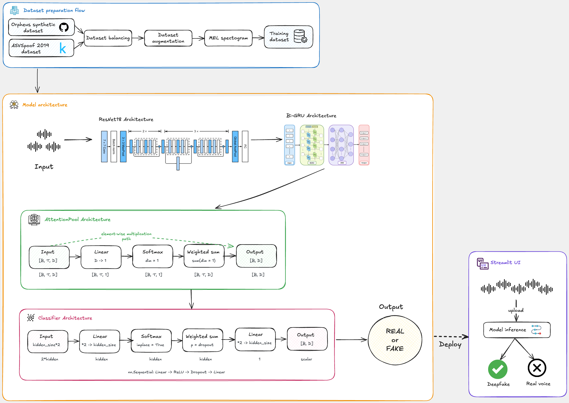
The main objectives in the following sections are to find and prepare the most suitable dataset, implement a detection model, train the model on the dataset and deploy it on a simple Streamlit interface.

This flow diagram illustrates all of the above steps:

So, what are we waiting for? Let’s dive into the data preparation step and get started!

---

3. Preparing the dataset

"The most sophisticated of the algorithms will fail to produce reliable results if they do not receive high quality and relevant data."

If your data does not point towards your goal, it is useless. When training an AI, you should first have a clear and reliable dataset.

Why is it important to have clear, representative datasets?

The answer lies in the problem we are trying to solve: we need to implement an algorithm that can detect whether an audio file is fake or real. To do this, we need a dataset containing enough fake and real audio files to enable us to predict whether a given input audio file is fake or real.

For this approach, we will use the ASV Spoof 2019 dataset, which contains a diverse collection of audio samples including genuine human speech, as well as AI-generated or spoofed audio.

Designed specifically to support research in ASV spoofing detection, the dataset includes attacks such as text-to-speech (TTS), voice conversion (VC) and replay attacks.

This dataset is divided into two categories: Logical Access (LA) and Physical Access (PA). Both are useful, but for our use case, the PA dataset is more useful. However, we will combine them to create a more robust dataset.

In addition to the ASV Spoof 2019 dataset, we will use some audio files generated using Orpheus to capture more realistic deepfake audio. (Don’t worry, those audio files will be provided for you)

Data Augmentation and Dataset Balancing

Now that we have a dataset, we need to prepare it for our model to ensure we get good, precise predictions.

How balanced is the dataset? After extracting all the audio files from the ASV Spoof 2019 dataset and adding up the ones generated by us we get:

bonafide(real audio files): 41373

spoof(fake audio files): 298668

This means that our dataset is imbalanced and needs balancing.

To achieve this, we will select the most relevant fake audio files (The ones generated by us, and as much data as possible from the PA files) for our use case and remove the other ones so that we have a equal amount of data on both sides.

import numpy as np
import random
import torch
import torchaudio
import torchaudio.transforms as transforms
import matplotlib.pyplot as plt

datasets = [...] # Here, you can add the paths to your dataset. 

# Separate fake audio files into PA, LA and Orpheus sources
fake_pa = []
fake_la = []
fake_Orpheus = []
real = []

def parse_labels_with_path(label_file_path, data_path):
    data = []
    with open(label_file_path, 'r') as f:
        for line in f:
            parts = line.strip().split()
            file_name = parts[1]
            label = 1 if parts[-1] == "bonafide" else 0
            file_path = os.path.join(data_path, file_name + ".flac")
            data.append((file_path, label))
    return data

for dataset in datasets:
    data = parse_labels_with_path(dataset['label_file'], dataset['data_path'])
    for file_path, label in data:
        if label == 1:
            real.append((file_path, label))
        else:
            if "PA" in dataset['label_file']:
                fake_pa.append((file_path, label))
            elif "LA" in dataset['label_file']:
                fake_la.append((file_path, label))
            else:
                fake_Orpheus.append((file_path, label))

# Shuffle the data
np.random.shuffle(real)
np.random.shuffle(fake_pa)
np.random.shuffle(fake_la)

np.random.seed(42)

# Calculate how many fakes we need.(70% PA and 30% LA)
n_real = len(real)
n_fake_pa = int(n_real * 0.7)
n_fake_la = n_real - n_fake_pa  # remaining 30%

# Ensure we don't sample more than available. (Here is not the case)
n_fake_pa = min(n_fake_pa, len(fake_pa))
n_fake_la = min(n_fake_la, len(fake_la))

# Random sampling. 
# Provides an array containing a specific number of samples from a given list of labelled audio files.
fake_pa_sample = random.sample(fake_pa, k=n_fake_pa)
fake_la_sample = random.sample(fake_la, k=n_fake_la)

# Combine all and shuffle
fake_Orpheus = os.listdir("Orpheus")
fake_Orpheus = [(os.path.join("Orpheus", file), 0) for file in fake_Orpheus]

balanced_data = real + fake_pa_sample + fake_la_sample + fake_Orpheus
random.shuffle(balanced_data)

# Separate paths and labels
X_balanced = np.array([x[0] for x in balanced_data])
y_balanced = np.array([x[1] for x in balanced_data])

OK, once this process is completed, we need to augment our data to cover a wider range of use cases. For this part, we need to define some functions that will perform these actions on our audio file.

class AudioUtil:
    @staticmethod
    def open(audio_file):
        sig, sr = torchaudio.load(audio_file)
        return sig, sr

    @staticmethod
    def rechannel(aud, new_channel):
        sig, sr = aud
        if sig.shape[0] == new_channel:
            return aud
        if new_channel == 1:
            resig = sig[:1, :]
        else:
            resig = sig.repeat(new_channel, 1)
        return resig, sr

    @staticmethod
    def resample(aud, newsr):
        sig, sr = aud
        if sr == newsr:
            return aud
        num_channels = sig.shape[0]
        resig = transforms.Resample(sr, newsr)(sig[:1, :])
        if num_channels > 1:
            retwo = transforms.Resample(sr, newsr)(sig[1:, :])
            resig = torch.cat([resig, retwo], dim=0)
        return resig, newsr

    @staticmethod
    def pad_trunc(aud, max_ms):
        sig, sr = aud
        num_rows, sig_len = sig.shape
        max_len = sr // 1000 * max_ms
        if sig_len > max_len:
            sig = sig[:, :max_len]
        elif sig_len < max_len:
            pad_begin_len = random.randint(0, max_len - sig_len)
            pad_end_len = max_len - sig_len - pad_begin_len
            pad_begin = torch.zeros((num_rows, pad_begin_len))
            pad_end = torch.zeros((num_rows, pad_end_len))
            sig = torch.cat((pad_begin, sig, pad_end), dim=1)
        return sig, sr

    @staticmethod
    def time_shift(aud, shift_pct):
        sig, sr = aud
        _, sig_len = sig.shape
        shift_amt = int(random.random() * shift_pct * sig_len)
        return sig.roll(shift_amt), sr

    @staticmethod
    def add_noise(aud, noise_level=0.005):
        sig, sr = aud
        noise = torch.randn_like(sig) * noise_level
        return sig + noise, sr

    @staticmethod
    def change_gain(aud, gain_db_range=(-6, 6)):
        sig, sr = aud
        gain_db = random.uniform(*gain_db_range)
        gain = 10 ** (gain_db / 20)
        return sig * gain, sr

    @staticmethod
    def pitch_shift(aud, n_steps=2):
        sig, sr = aud
        return torchaudio.functional.pitch_shift(sig, sr, n_steps), sr

A brief description of each defined function:
open(audio_file) - just returns the waveform and the sample rate of the audio file

rechannel(aud, newchannel) - makes the audio signal into a 1 channel(mono) or 2 channel(stereo) audio file depends on newchannel.

resample(aud, newsr) - It changes the sample rate of the audio signal if it is different to the new sample rate.

pad_trunc(aud, max_ms) - Truncates the audio signal to the specified maximum duration (max_ms).

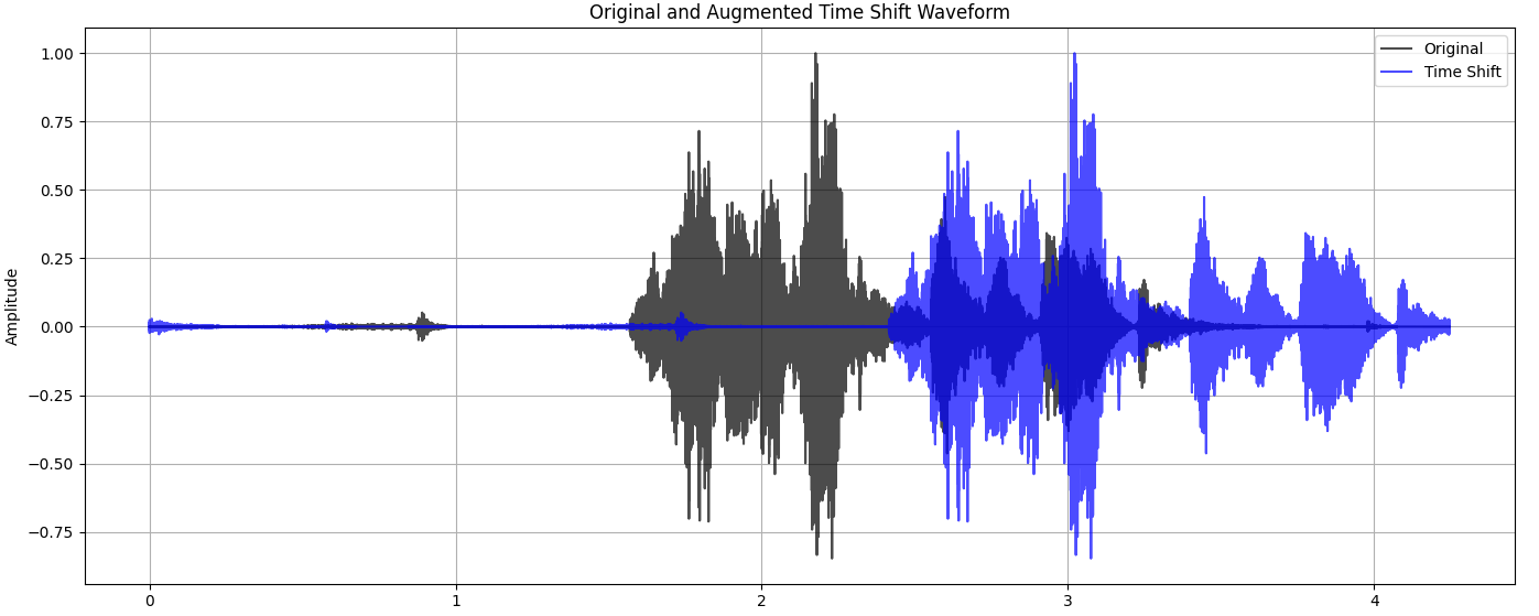
time_shift(aud, shift_pct) - shifts the audio signal forward or backward in time by a random amount(within a percentage of the total length ).

add_noise(aud, noise_level = 0.005) - adds noise to the audio signal.

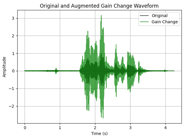
change_gain(aud, gain_db_range=(-6, 6)) - increses the db of the audio signal.

pitch_shift(aud, n_steps=2) - It modifies the pitch of the audio signal by a specified amount of semitones(n_steps).

Visualizing the Impact of Augmentation

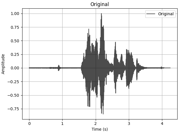
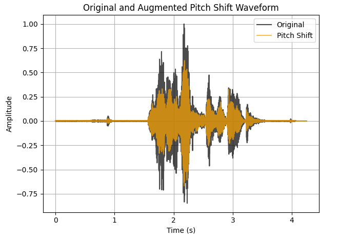
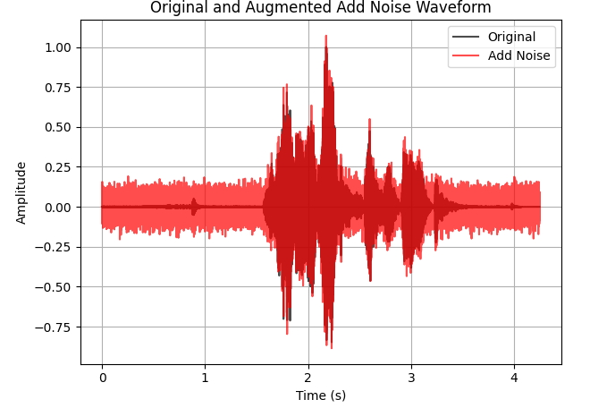
Before we move on to feature extraction, it’s important to compare our augmented data with the original. Although these changes may not seem significant, they have a substantial impact on our model's ability to generalize.

Here are some examples of augmented versions of our original audio file:

Original audio:

Time shifted audio:

Gain Changed audio:

Pitch Shifted audio:

Audio with added noise:

Feature Extraction

We have the dataset, but we still need to convert our audio into a format that neural networks can easily understand.

Feeding raw waveforms to our model is often inefficient and computationally expensive, even though it works. However, let's not do that.

So, what kind of feature extraction are we going to use? And which format would be the best fit for our needs?

This is indeed a complicated question, especially since there are different types of feature extraction that work with raw data. To answer it, we need to compare the different approaches and see which one fits our requirements.

To make this comparison, I used six different feature extraction techniques that had previously been used in ASV challenges.

Here is a table comparing all six feature extraction techniques, along with their respective pros and cons, brief descriptions, and optimal applications:

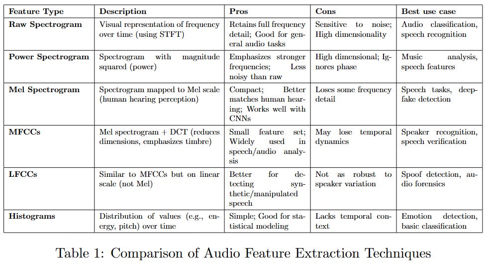
As can be seen in the table, the Mel spectrogram and LFCC feature extraction would be the perfect fit for our implementation.

Considering the limitations of converting the LFCC back to an audio file, we will only use the Mel spectrogram from now on.

Perhaps implementing a hybrid approach by combining the two would be a good idea to achieve better results. For now, though, we will proceed as planned.

Now that we have found the best match for our feature extraction, we can continue by updating our AudioUtil class with two more functions.

Those functions will generate the spectrogram we need from the audio sample or add a new augmentation feature to the generated spectrogram.

This feature will mask a specific portion of the spectrogram, either in time or frequency. We will see an example of this later on.

For now, these are the two newly added functions:

    @staticmethod
    def spectro_gram(aud, n_mels=64, n_fft=780, hop_len=195):
        sig, sr = aud
        spec = transforms.MelSpectrogram(sr, n_fft=n_fft, hop_length=hop_len, n_mels=n_mels)(sig)
        spec = transforms.AmplitudeToDB(top_db=80)(spec)
        return spec

    @staticmethod
    def spectro_augment(spec, max_mask_pct=0.1, n_freq_masks=1, n_time_masks=1):
        _, n_mels, n_steps = spec.shape
        mask_value = spec.mean()
        aug_spec = spec
        freq_mask_param = int(max_mask_pct * n_mels)
        for _ in range(n_freq_masks):
            aug_spec = transforms.FrequencyMasking(freq_mask_param)(aug_spec, mask_value)
        time_mask_param = int(max_mask_pct * n_steps)
        for _ in range(n_time_masks):
            aug_spec = transforms.TimeMasking(time_mask_param)(aug_spec, mask_value)
        return aug_spec

Before we proceed with the implementation, it would be helpful to explain the purpose of each argument in the spectro_gram function and provide some sample spectrograms for visual reference, as well as an example of an augmented spectrogram created using the spectro_augment function.

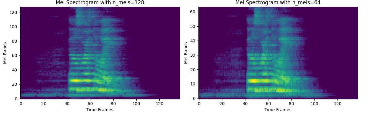
n_mels
The n_mels argument specifies the number of Mel filter banks to be generated. More bins result in a finer resolution on the Mel scale. We will therefore use 64 bins to achieve clear resolution and avoid overfitting during training.

This is because a spectrogram with richer frequency details causes the model to focus too closely and prevents it from generalising when given other audio files.

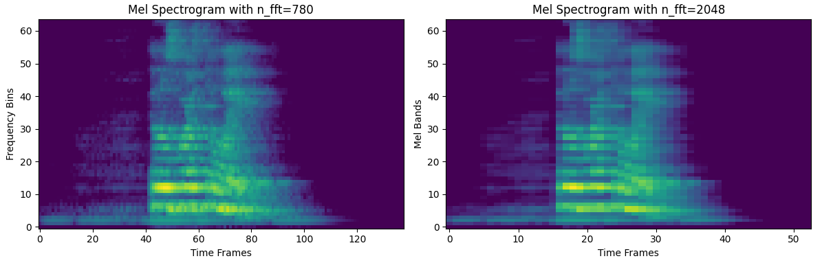
n_fft

The value of n_fft determines the resolution of frequency axis. In theory, the higher n_fft value, the higher the resolution, but in reality, this doesn't seem to be the case. Therefore, when you visualise it, it might look more blurry, even though the resolution is finer.

The best approach here is to select the most appropriate n_fft value, i.e. one that doesn’t blur our image to such an extent that we encounter overfitting issues, but which is also large enough to capture the important information required by our model.

That’s why we will choose a value between the most commonly used ones (512 and 1024) to ensure good generalisation. The value will be 780.

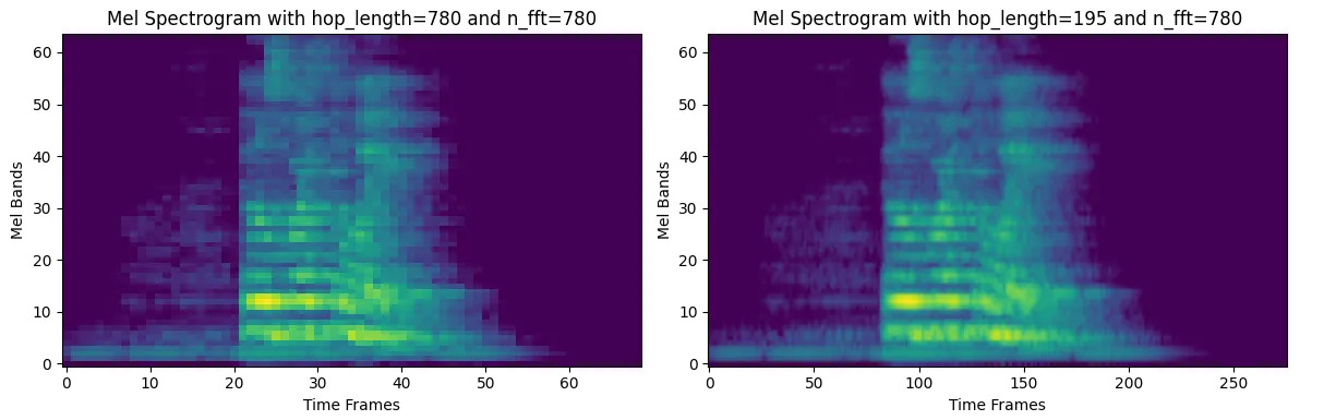
hop_len

The hop_len determines the resolution of the time axis. The value of n_fft // 4 is used by default.

In general, the value of hop_len is low because it provides better time resolution and more temporal detail, at the cost of higher computational efficiency compared to a much higher value.

Therefore, we will use a hop length of n_fft // 4, as this is widely used for speech and general audio.

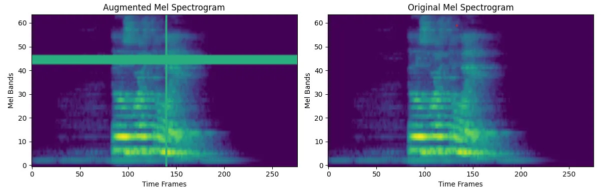
Example of augmented spectogram

Calling spectro_augment with generate_spectrogram will produce an augmented Mel spectrogram with two(or more) masked segments on the horizontal (time) and vertical (frequency) axes.

This allows us to cover distorted audio files with missing fragments.

Adding it all up

We have implemented all the necessary functions to augment the data and transform every audio file into a Mel spectrogram. Now we need to apply these functions to our balanced dataset.

To achieve this, we will create a class containing all the defined functions and returning all the generated spectrograms with their respective labels.

Before we start working on the code, let's take a step back and review the workflow we're going to use for preparing the data.

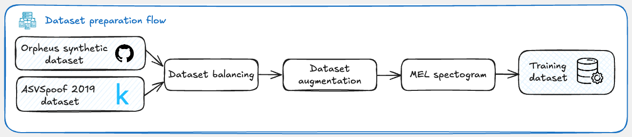
Now that the workflow is complete, we can start bringing everything together by implementing a class that will prepare the dataset for us.

from torch.utils.data import DataLoader, Dataset, random_split

class SoundDS(Dataset):
    def __init__(self, data_path, label, mode="original"):
        self.label = label
        self.data_path = [str(p) for p in data_path]
        self.duration = 4000
        self.sr = 16000
        self.channel = 2
        self.shift_pct = 0.4
        self.mode = mode

    def __len__(self):
        return len(self.data_path)

    def __getitem__(self, idx):
        audio_file = self.data_path[idx]
        class_id = self.label[idx]

        aud = AudioUtil.open(audio_file)
        aud = AudioUtil.resample(aud, self.sr)
        aud = AudioUtil.rechannel(aud, self.channel)
        aud = AudioUtil.pad_trunc(aud, self.duration)

        if self.mode == "time_shift":
            aud = AudioUtil.time_shift(aud, self.shift_pct)
        elif self.mode == "add_noise":
            aud = AudioUtil.add_noise(aud, noise_level=random.uniform(0.005, 0.05))
        elif self.mode == "pitch_shift":
            aud = AudioUtil.pitch_shift(aud, n_steps=random.randint(1,3))
        elif self.mode == "combined":
            aud = AudioUtil.time_shift(aud, self.shift_pct)
            aud = AudioUtil.add_noise(aud, noise_level=random.uniform(0.005, 0.05))

        sgram = AudioUtil.spectro_gram(aud, n_mels=64, , n_fft=780, hop_len=195)

        if self.mode in ["spectro_augment", "combined"]:
            sgram = AudioUtil.spectro_augment(sgram, max_mask_pct=0.1, n_freq_masks=random.randint(1,3), n_time_masks=random.randint(1,3))

        return sgram, class_id

This class contains all the functions required to augment our dataset and generate the spectrogram. Now, we can simply call it with the specific mode to augment it as required.

from torch.utils.data import random_split, ConcatDataset

original_ds = SoundDS(X_balanced, y_balanced, mode="original")
time_shift_ds = SoundDS(X_balanced, y_balanced, mode="time_shift")
noise_ds = SoundDS(X_balanced, y_balanced, mode="add_noise")
pitch_shift_ds = SoundDS(X_balanced, y_balanced, mode="pitch_shift")
spectro_aug_ds = SoundDS(X_balanced, y_balanced, mode="spectro_augment")
combined_ds = SoundDS(X_balanced, y_balanced, mode="combined")

full_augmented_dataset = ConcatDataset([original_ds, time_shift_ds, noise_ds, spectro_aug_ds, combined_ds, pitch_shift_ds])

Our dataset is ready for training!

---

Coming Up Next: Model Training & Deployment

In the following article, we’ll discuss about the exciting part of seeing the final dataset be put to work!

A breakdown of what’s coming:

• We’ll be using a pre-trained ResNet18 model with Bi-GRU to classify the audio.

• Show you how we got to 95-97% precision & recall in less epochs, what worked and what didn’t.

• How to build a Streamlit app that allows real-time inference: users upload audio files, which are preprocessed and classified as REAL or FAKE with confidence scores.

🔗 Check out the code on GitHub and support us with a ⭐️